Getting Started 2

Update date:

Forewords

This document completes the first Getting Started tutorial. It aims at explaining how to implement an application with MECSYCO framework using most of the functionality describe in the User Guide section. It still focuses on how to code the launchers.

Some knowledge about multi-modeling, the MECSYCO concepts and the Java programming language could be helpful. This time we will study the Lorenz system. To learn more about the Lorenz system, please refer to the Wikipedia article about Lorenz.

The environment used in this tutorial is Eclipse 4.16.0 with the Java Development Kit 1.8.

Setup

You can follow the Getting Started 2 in the MecsycoScholar project just like for Getting Started tutorial. Follow the same steps for the import.

The final code of this tutorial is available in the mecsycoscholar.application.gettingstarted2 package.

Table of Contents

Chapter Description  
My first multi-model: the Lorenz system   Description of the example studied: Lorenz system
Programming a Lorenz multi-model   Basic launcher construction from the scratch
Simulation with different time steps   Bonus: multiple time steps work!
Adding observation to simulations and SimulData manipulation   Use of MECSYCO-visu. Create SimulData and manipulate a model artifact
Using the distributed version   Use of MECSYCO-com-dds (coupling with MECSYCO-visu)
Using FMUs   Use of MECSYCO-world-fmi (coupling with MECSYCO-visu and the multiplexer)

My first multi-model: the Lorenz system

Viewing Lorenz system as a multi-model

We suppose 3 models, one for each variable named respectively X, Y and Z. As a consequence, the multi-model makes use of 3 agents AgentX, AgentY and AgentZ, each respectively associated to the management of one variable.

Each agent is associated to a simulator (here it is a differential equation solver). Each simulator (and by extension each agent) is defined by:

  1. Its inputs: the name of incoming information
  2. Its outputs: the name of outgoing information

For example the model corresponding to the evolution of the Y variable needs as input, the value of X and Z, and provides the Y value as output. For clarity reason, Y denotes the same information whatever the simulator or agent.

The equations depend on some initial parameters that are here called A, B and C.

Synthesis:

3 agents:

  1. AgentX defined by:
    • output X the value of the X variable
    • input Y
    • parameter a (A in the code)
    • initial value init_X
  2. AgentY defined by:
    • output Y the value of the Y variable
    • input X and Z
    • parameter b (B in the code)
    • initial value init_Y
  3. AgentZ defined by:
    • output Z the value of the x variable
    • input X and Y
    • parameter c (C in the code)
    • initial value init_Z
Lorenz multi-model
Figure 2: Lorenz multi-model

Programming a Lorenz multi-model


The multi-model in MECSYCO is built at the same time as the launcher. The following steps need to be achieved in order to obtain a multi-model:

  • Creating the agents
  • Creating their simulators
  • Creating their model artifact and connect them to the corresponding agents
  • Creating the communication links and use them to connect the agents

Assumptions

Assumption 1: The 3 simulators LorenzX, LorenzY and LorenzZ are provided. They contains in addition to the original, rudimentary trace functionalities to observe simulation. At each step of resolution, the solver prints in the console the current time step, the name of the agent and the set of values of its variables (Figure 3).

rudimentary trace
Figure 3: Console trace


Each simulator is a Java class and implements an Euler solver (also provided under the name Equation); its constructor takes as parameters the initial value of the variable and the value of its parameter.

Assumption 2: The model artifact to use is already implemented and provided as the Java class EquationModelArtifact. In order to manage one of the simulators, you needs to create one instance of this class by providing a name that informs about the simulator it manages (it is not mandatory, but permits a better code display) and the simulator instance.

For more information about model artifact, see User Guide section “The interface artifact”.

Assumption 3: We will use the following values as parameters of the simulation:


// --- simulation time
double maxSimulationTime = 100;

//initial values of variables
double init_X =1, init_Y =1, init_Z =4;

//parameter values of equation
double A = 10, B =28, C =2.67;
Code 1: Parameters of the simulation

Before you start, create a new Java class in the Launcher package created at this purpose. This class will contains our main for the multi-model and launcher. In the main, you can already add the previous code lines.

Create the 3 agents


EventMAgent AgentX = new EventMAgent("agentX", maxSimulationTime);
EventMAgent AgentY = new EventMAgent("agentY", maxSimulationTime);
EventMAgent AgentZ = new EventMAgent("agentZ", maxSimulationTime);
Code 2: Creation of the 3 agents

Create the simulators

Here, we are only instantiating the solver. The link with the agent is done thanks to the model artifact:


LorenzX SimulatorX= new LorenzX(init_X, A);
LorenzY SimulatorY= new LorenzY(init_Y, B);
LorenzZ SimulatorZ= new LorenzZ(init_Z, C);
Code 3: Creation of the 3 simulators

Create the artifacts

Provide the model ID then the simulator. This is specific to this model artifact. These arguments depend on how you create the model artifact class. After each creation, you need to link it to the proper agent (by setting it):


EquationModelArtifact ModelArtifactX = new EquationModelArtifact("Xmodel", SimulatorX);
AgentX.setModelArtifact(ModelArtifactX);

EquationModelArtifact ModelArtifactY = new EquationModelArtifact("Ymodel", SimulatorY);
AgentY.setModelArtifact(ModelArtifactY);

EquationModelArtifact ModelArtifactZ = new EquationModelArtifact("Zmodel", SimulatorZ);
AgentZ.setModelArtifact(ModelArtifactZ);
Code 4: Creation and link to the agents of the 3 model artifacts

You need to create one link per directional communication (that is to say for each arrow of Figure 2 ). You need to instantiate the support (CentralizedEventCouplingArtifact) then the link by defining if it is the input or the output port and the name of the port (in our models, the name of the port, input or output, is the name of the value transmitted):


CentralizedEventCouplingArtifact XOutputToZ = new CentralizedEventCouplingArtifact();
AgentX.addOutputCouplingArtifact(XOutputToZ,"X");
AgentZ.addInputCouplingArtifact(XOutputToZ,"X");

CentralizedEventCouplingArtifact XOutputToY = new CentralizedEventCouplingArtifact();
AgentX.addOutputCouplingArtifact(XOutputToY,"X");
AgentY.addInputCouplingArtifact(XOutputToY,"X");

CentralizedEventCouplingArtifact YOutputToX = new CentralizedEventCouplingArtifact();
AgentY.addOutputCouplingArtifact(YOutputToX,"Y");
AgentX.addInputCouplingArtifact(YOutputToX,"Y");

CentralizedEventCouplingArtifact YOutputToZ = new CentralizedEventCouplingArtifact();
AgentY.addOutputCouplingArtifact(YOutputToZ,"Y");
AgentZ.addInputCouplingArtifact(YOutputToZ,"Y");

CentralizedEventCouplingArtifact ZOutput = new CentralizedEventCouplingArtifact();
AgentZ.addOutputCouplingArtifact(ZOutput,"Z");
AgentY.addInputCouplingArtifact(ZOutput,"Z");
Code 5: Creation of the links between agents

Launching the simulation

Now the whole multi-model is described. The launcher part is the remaining part of the main. We need to start the simulation softwares, initialize them and run them. Since a simulator is part of the software, all action will be done with the agents. In some case, you can also set the model parameters but here we won’t need to do it.

First then, start of the model softwares:


AgentX.startModelSoftware();
AgentY.startModelSoftware();
AgentZ.startModelSoftware();
Code 6: Starting the model softwares


Next is to initialize the co-simulation. That is to say make the simulators share their values. This action need to be in a try and catch section of the code:


try{
  AgentX.coInitialize();
  AgentY.coInitialize();
  AgentZ.coInitialize();
}
catch(CausalityException e){
  e.printStackTrace();
}
Code 7: Initialize the co-simulation


Then start the simulation:


AgentX.start();
AgentY.start();
AgentZ.start();
Code 8: Starting the simulation


You should see in the console somthing like the figure 3. The user does not need to synchronize simulators, MECSYCO does it. To understand deeper, refer to User Guide Appendix C, or look for the Chandy-Misra-Bryant algorithm.

Comments

We are using a default time step (0.01) for all solver.
We are simply building a simple launcher here, we are not using any visualization tool or DDS.

Simulation with different time steps


Our simulators have a second constructor that allows us to define the time step. It is then possible to have the three simulators with different time step, and MECSYCO will still manage synchronization without trouble. Then, if we use code 9 for the simulator construction:


LorenzX SimulatorX= new LorenzX(init_X, A, 0.01);
LorenzY SimulatorY= new LorenzY(init_Y, B, 0.02);
LorenzZ SimulatorZ= new LorenzZ(init_Z, C, 0.07);
Code 9: Creation of the simulator using the second constructor


Then we obtain the following result:

Multiple time step result
Figure 4: Result with multiple time step


Explanation: at first, only the Xmodel is working, but if you look at the Lorenz system, X variation is influenced by the difference between X and Y. This is why there is no movement since Xmodel don’t know the new value of Y yet.

Ymodel will only send its new value each 0.02 simulation time. Between these 0.02 Xmodel will evolve freely with its current value of Y (time step 0.03 and 0.04) and Y won’t move.

The same go for Z, it will not influence Y and be influenced by X and Y until 0.07.

These points are the different discretization for X, Y and Z, and we show that we can defined different time discretization for each solver in order to match the best one for each, and MECSYCO will manage the synchronization.

Adding observation to simulations and SimulData manipulation


Here, we will show how to use the visualization tool of MECSYCO . You will first need to add in your project the MECSYCO-visu jar and the dependencies (jfreechart, JCommon, Jzy3d 0.9.1, Gluegen and JOGL).

We will also manipulate the model artifact in order to create special output for the observer.

You can use any time step, but for better results, the default time step is advised.

For detailed information, see User Guide MECSYCO-visu.

Agent, dispatcher and connection

The observer is used as any other agent, but we give it the capacity to get more than one model artifact thanks to a dispatcher. For the first step, you need to create the observing system (agent and dispatcher):


ObservingMAgent obs=new ObservingMAgent("obs",maxSimulationTime);
SwingDispatcherArtifact Dispatcher=new SwingDispatcherArtifact();
obs.setDispatcherArtifact(Dispatcher);
Code 10: Creation of the observing system


Then you can connect the output port of the Lorenz agents to our observer like we did before for connecting the agents.

Add of special outputs

Some observing artifact need specific SimulData to work. We will now create specific ports where the usual data will be converted to the correct SimulData we need, i.e. a Tuple3 of Double values, a SimulVector of Double values, and a Tuple2 of Double values (cf User Guide section “Simulation data” or SimulData manipulation ).

Take a look to our model artifact (EquationModelArtifact) at the method named getExternalOutputEvent. This is where we manage the outputs of our model in order to create output ports. As you can see, 3 condition were not filled. They are our new outputs port (obs2D, obs3d and obsVector).

obs2D

We need to create a Tuple2 filled with real values. We will try to catch the X and Y values, to do this we have the method getVariable contains in the model (Equation). We can now create the event that will contains those values under the form of a Tuple2, with a time stamp:


final Double x=equation.getVariable("X");
final Double y=equation.getVariable("Y");

result=new SimulEvent(new Tuple2<>(x,y), equation.getTime());
Code 11: obs2D section

obs3d

This time we need a Tuple3. This is the same process as before, but we add the Z value.

obsVector

Lastly, we need a SimulVector, but as the guide said, the constructor is contained in the Java class ArrayedSimulVector. This vector will contain the value of X, Y and Z:


final Double x=equation.getVariable("X");
final Double y=equation.getVariable("Y");
final Double z=equation.getVariable("Z");

result=new SimulEvent(new ArrayedSimulVector<>(x,y,z), equation.getTime());
Code 12: obsVector section

else

This condition is already filled. It allows the user to use any kind of port’s name, but due to the method getVariable, only X, Y and Z can really work (state variable of the model).

Notes

The Z value is not contained in every model (LorenzX do not), so only agents’ link to LorenzY and LorenzZ can use the last two output ports.

You can now use them now to create the links (AgentX to obs with obs2D, AgentZ to obs with obs3d and obsVector for example).

Of course, obs is also an agent so at the end of the main, a startModelSoftware and a start are mandatory.

Graphics

You can now use all graphics available in MECSYCO-visu! But how?
Try to add code 13 after the new links you have created:


Dispatcher.addObservingArtifact (
  new LiveTXGraphic ("Lorenz temporal", "Value", Renderer.Line,
  new String [] {"SeriesX", "SeriesY", "SeriesZ"},
  new String [] {"X", "Y", "Z" }));

Dispatcher.addObservingArtifact (
  new LiveXYGraphic("Lorenz phase", "X", "Y", Renderer.Line, "XY", "XY"));

Dispatcher.addObservingArtifact (
  new LiveBarGraphic("Lorenz bar", "Bars", "Value", 
  new String [] {"X", "Y", "Z"}, "XYZVector"));

Dispatcher.addObservingArtifact (
  new LivePieGraphic("Lorenz Pie", new String [] {"X", "Y", "Z"}, "XYZVector"));

Dispatcher.addObservingArtifact (
  new LiveEventGraphic("Lorenz factual", "time", "X", "X", "X"));

Dispatcher.addObservingArtifact (
  new Live3DGraphic("Lorenz 3D", "X", "Y", "Z", "XYZ"));

Code 13: Creation of the observing artifacts for the graphs


In this code we named the input of the observing agent following this mapping:

  • input “X” link to AgentX output
  • input “Y” link to AgentY output
  • input “Z” link to AgentZ output
  • input “XY” link to the agent using output “obs2D”
  • input “XYZ” link to the agent using output “obs3d”
  • input “XYZVector” link to the agent using output “obsVector”

As you can see, it is not mandatory here to have the same names for input and output, only the same CentralizedEventCouplingArtifact is needed. Nice graphics you have there, no? (Figure5) In all this case, we used the live version of our graphics as a consequence, the simulation take more time than before. In order to avoid this issue, it is advised to use the postmortem version of the graphs (replace Live by PostMortem).

All graphs
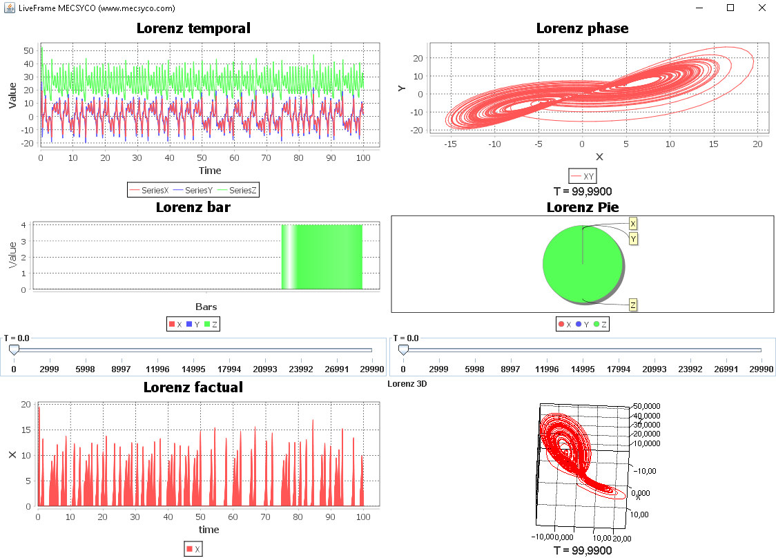
Figure 5: All graphs

Post treatment

The visualization package does not only contain visualization tool, but post treatment tool too.

Data comparator

One of them is the data comparator. It will compare the result of the simulation with data sheets. For the Lorenz case, the data sheets with the right format are already provided. You only need to turn on the Debug system, and put it in info mode. To do so, thanks to your project explorer, go to the file mecsyco.properties in the folder conf, and make sure you have the following configuration:


# 1. Logging configuration
# 1.1 Logging level

# level order: off < error < warn < info < debug < trace < all

ROOT_LOGGING_LEVEL=info

# Use `inherited' value for using ROOT_LOGGING_LEVEL
M_AGENT_LOGGING_LEVEL=inherited
INTERFACE_LOGGING_LEVEL=inherited
COUPLING_LOGGING_LEVEL=inherited


# 1.2 Logging output

# Comment/Uncomment for enabling/disabling console or file logging

CONSOLE_LOGGING_ENABLED
# FILE_LOGGING_ENABLED


# 1.3 Other

ASYNC_LOGGING_ENABLED

LOGGING_FILE_PATH=./log

# %thread Thread name
# %level Logging level
# %logger Logger name
# %marker Logging marker
# %message Logging message
# %date ISO-8601 date
# %relative Elapsed time since the application starting
# %n New line
LOGGING_PATTERN=[%thread] %level %logger -- %message%n
Code 14: Mecsyco debug system properties

Now, everything is ready so let just try code 15 and see what the console has to say (Figure 6):


Dispatcher.addObservingArtifact (
  new DataComparator(
  new String[] { "resources/model_checking/lorenzLog_x.csv", "resources/model_checking/lorenzLog_y.csv","resources/model_checking/lorenzLog_z.csv"} ,
  new String[] { "X", "Y", "Z" }));
Code 15: Creation of the observing artifact for data comparator


Comparator result
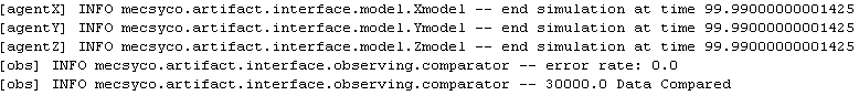
Figure 6: Comparator result

Logging

The package also contains a logging system, which means that you can save your result in external files. The logging can be done by creating one file per output you need to log, or by creating one for all:


String path="data_log/";

//Dispatcher.addObservingArtifact (new LoggingArtifact (
 //new String[] {path+"X.csv",path+"Y.csv",path+"Z.csv"}, 
 //new String [] {"Xobs","Yobs","Zobs"}, "%time;%value\n"));
Dispatcher.addObservingArtifact (new LoggingArtifact (
  path+"X.csv", new String [] {"X"}, "%time;%value\n"));
Dispatcher.addObservingArtifact (new LoggingArtifact (
  path+"Y.csv", new String [] {"Y"}, "%time;%value\n"));
Dispatcher.addObservingArtifact (new LoggingArtifact (
  path+"Z.csv", new String [] {"Z"}, "%time;%value\n"));
  
Dispatcher.addObservingArtifact (new LoggingArtifact (
  path+"XYZ.csv", new String [] {"XYZ"}, "%time;%value\n"));

Dispatcher.addObservingArtifact (new LoggingArtifact (
  path+"result.csv", new String [] {"X", "Y", "Z", "XYZ"}, "%time;%value\n"));
  
Dispatcher.addObservingArtifact (new LoggingArtifact (
  path+"multi.csv", new String [] {"X", "Y", "Z", "XYZ"}, "%time;%value\n",
  new String[]{"X_Tuple2_1","X_Tuple2_2","Y_Tuple2_1","Y_Tuple2_2","Z_Tuple2_1","Z_Tuple2_2","XYZ_Tuple3_1","XYZ_Tuple3_2","XYZ_Tuple3_3"}, 
  false));
Code 16: Creation of the observing artifact for the logs


Since no agent have an output port that provide a simple Tuple1 containing the output value, we have to use the alternative option to create one file per output (line 7 to 12). You are free to create the output ports Xobs, Yobs and Zobs yourself and try the commented code (it means that the inputs of the observer are also named Xobs, Yobs and Zobs)! As the result you should have the following file created in data_log:

Files created Results
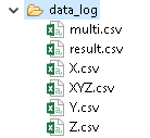
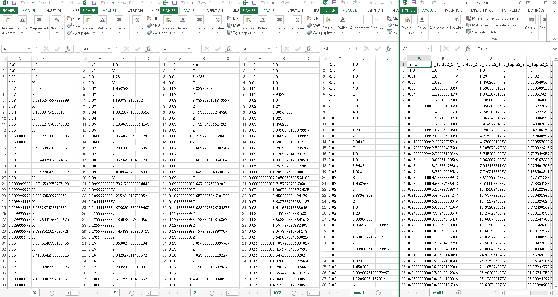
Figure 7: Files created and content

Analyze with R

The last functionality of MECSYCO-visu is the possibility to launch an R script in order to treat your result. This functionality is not optimal yet:

  • When installing R, choose a file with a path without space or special character
  • File path (of the file to treat) as to be define in the script

Dispatcher.addObservingArtifact (new LogToRProject (
  path+"ResultR2.csv", new String[]{"X","Y","Z"}));
Code 17: Creation of the model artifact for launching R script


Rscript.exe R file to launch
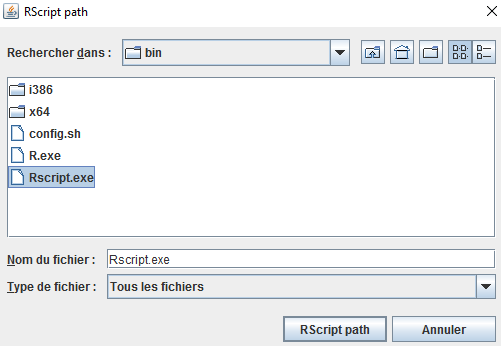
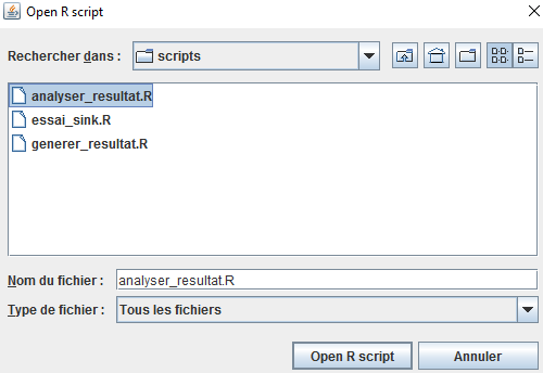
Figure 8: R launcher


ResultR2.csv is a file created by LogToRProject using the ports given (here X, Y, Z). This file can be use by your Rscript. In this example, we already provide you a script (DemoR.R) that will analyze the file named “result.csv”” in the folder “data_log” and create a file named “ResultR.csv” in the same folder. This Script will give the min and max value of each column, and the mean value. The csv to treat with this script follow the following structure:

  • Without header
  • The first column is not analyzed, so it could be the name, or the time step
  • The others columns contain only real values
  • Column separator are “;” and decimal separator are “.”

The results will also be found in “data_log”:

Files created Results
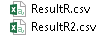
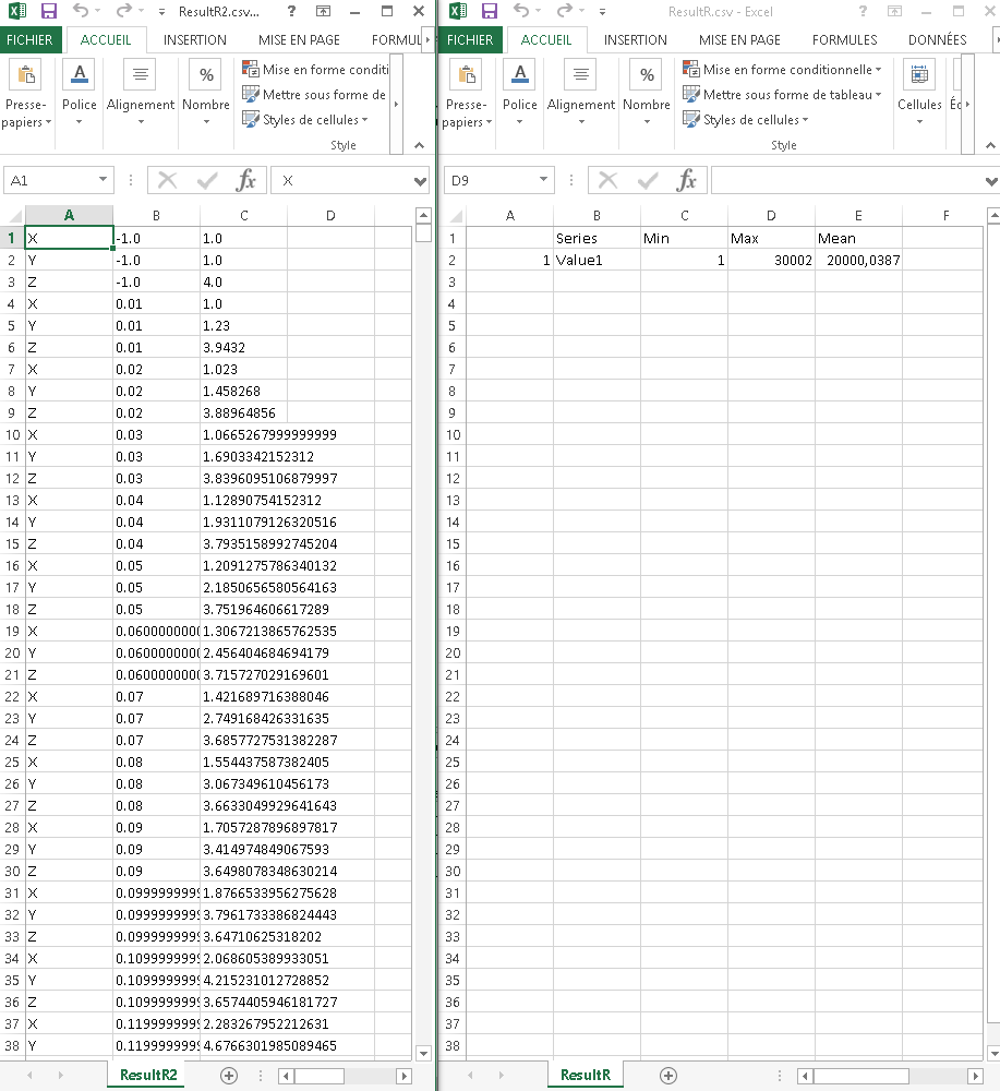
Figure 9: Files created and content (R)

Using the distributed version


We will now use the MECSYCO-com-dds package in order to distribute the model. You will then need to add the corresponding jar to your project (dependencies: Opensplice DDS community edition 6.4 and Jackson databind).

For detailed information, see MECSYCO-com-dds. This guide can also help you install properly Opensplice DDS.

One launcher per model

We will distribute the Lorenz model following figure 10

Decentralized Lorenz
Figure 10: Lorenz decentralized

We will then have one launcher per model. We will also use our visualization tool in the Z Launcher (Live3DGraphic).

For each launcher you have to define:

  • Agents and artifacts like before
  • The data to send through DDS (DDSEventCouplingArtifactSender, red links)
  • The data received through DDS with the data type expected (DDSEventCouplingArtifactReceiver)
  • One sender implies one receiver! They are linked thanks to the topic (String in the constructor of the coupling)
  • The data not using DDS and defined as before (CentralizedCouplingArtifact, black link)
  • Start correctly all agent (startModelSoftware…)

LorenzXLauncher


double maxSimulationTime=100;
  	double init_X=1;
		double A=10;
		
		EventMAgent AgentX = new EventMAgent("agentX",maxSimulationTime);
		LorenzX SimulatorX=new LorenzX(init_X,A,0.01);
		EquationModelArtifact ModelArtifactX = new EquationModelArtifact ("Xmodel",SimulatorX);
		AgentX.setModelArtifact(ModelArtifactX);
		
		//output
		DDSEventCouplingArtifactSender XOutputToZ=new DDSEventCouplingArtifactSender("XtoZ");
		AgentX.addOutputCouplingArtifact(XOutputToZ,"X");
		DDSEventCouplingArtifactSender XOutputToY=new DDSEventCouplingArtifactSender("XtoY");		
		AgentX.addOutputCouplingArtifact(XOutputToY,"X");
		
		//Input
		DDSEventCouplingArtifactReceiver YOutputToX=new DDSEventCouplingArtifactReceiver("YtoX",Tuple2.of(Double.class, String.class));
		AgentX.addInputCouplingArtifact(YOutputToX,"Y");
		
		AgentX.startModelSoftware();
		
		try {
			AgentX.coInitialize();
		} catch (CausalityException e) {
			// TODO Auto-generated catch block
			e.printStackTrace();
		}
		AgentX.start();
Code 18: Launcher 1: AgentX

LorenzYLauncher


double maxSimulationTime=100;
  	double  init_Y=1;
		double B=28;
		
		EventMAgent AgentY = new EventMAgent("agentY",maxSimulationTime);
		LorenzY SimulatorY=new LorenzY(init_Y,B,0.01);
		EquationModelArtifact ModelArtifactY = new EquationModelArtifact ("Ymodel",SimulatorY);
		AgentY.setModelArtifact(ModelArtifactY);
		
		//output
		DDSEventCouplingArtifactSender YOutputToX=new DDSEventCouplingArtifactSender("YtoX");
		AgentY.addOutputCouplingArtifact(YOutputToX,"Y");
		DDSEventCouplingArtifactSender YOutputToZ=new DDSEventCouplingArtifactSender("YtoZ");
		AgentY.addOutputCouplingArtifact(YOutputToZ,"Y");
		
		
		//Input
		DDSEventCouplingArtifactReceiver XOutputToY=new DDSEventCouplingArtifactReceiver("XtoY",Tuple2.of(Double.class, String.class));		
		AgentY.addInputCouplingArtifact(XOutputToY,"X");
		DDSEventCouplingArtifactReceiver ZOutput=new DDSEventCouplingArtifactReceiver("Z",Tuple2.of(Double.class, String.class));
		AgentY.addInputCouplingArtifact(ZOutput,"Z");
		
		AgentY.startModelSoftware();
		
		try {
			AgentY.coInitialize();
		} catch (CausalityException e) {
			// TODO Auto-generated catch block
			e.printStackTrace();
		}
		AgentY.start();
Code 19: Launcher 2: AgentY

LorenzZLauncher


double maxSimulationTime=100;
  	double init_Z=4;
		double C=2.67;
		
		EventMAgent AgentZ = new EventMAgent("agentZ",maxSimulationTime);
		LorenzZ SimulatorZ=new LorenzZ(init_Z,C,0.01);
		EquationModelArtifact ModelArtifactZ = new EquationModelArtifact ("Zmodel",SimulatorZ);
		AgentZ.setModelArtifact(ModelArtifactZ);
		
		//output
		DDSEventCouplingArtifactSender ZOutput=new DDSEventCouplingArtifactSender("Z");
		AgentZ.addOutputCouplingArtifact(ZOutput,"Z");
		
		//Input
		DDSEventCouplingArtifactReceiver XOutputToZ=new DDSEventCouplingArtifactReceiver("XtoZ",Tuple2.of(Double.class, String.class));		
		AgentZ.addInputCouplingArtifact(XOutputToZ,"X");
		DDSEventCouplingArtifactReceiver YOutputToZ=new DDSEventCouplingArtifactReceiver("YtoZ",Tuple2.of(Double.class, String.class));		
		AgentZ.addInputCouplingArtifact(YOutputToZ,"Y");
		
		//Observing
		ObservingMAgent obs=new ObservingMAgent("obs", maxSimulationTime);
		SwingDispatcherArtifact Dispatcher=new SwingDispatcherArtifact();
		obs.setDispatcherArtifact(Dispatcher);
		
		CentralizedEventCouplingArtifact ZOutputTuple3ToObs=new CentralizedEventCouplingArtifact();
		AgentZ.addOutputCouplingArtifact(ZOutputTuple3ToObs, "obs3d");
		obs.addInputCouplingArtifact(ZOutputTuple3ToObs, "XYZ");
		
		Dispatcher.addObservingArtifact (
				new Live3DGraphic("Lorenz 3D", "X", "Y", "Z", "XYZ"));
		
		AgentZ.startModelSoftware();
		obs.startModelSoftware();
		
		try {
			AgentZ.coInitialize();
		} catch (CausalityException e) {
			// TODO Auto-generated catch block
			e.printStackTrace();
		}
		AgentZ.start();
		obs.start();
Code 20: Launcher 3: AgentZ

Here you are ready. You can test it in local by launching one after another each launcher. In order to decentralized it, each computer need the full installation (MECSYCO-re, MECSYCO-com-dds. MECSYCO-visu only if you use it) then you just need to launch the launchers (one per computer, two in the same and the last in another computer, as you want). The result should be display on the screen of the computer launching LorenzZLauncher and it is under the form of a graph 3D (see Figure 5 (Lorenz 3D)).

Using FMUs

We will now use FMUs to build our launcher, to do so, we will use MECSYCO-world-fmi package (currently in the Beta section of our site) with the dependencies: FMU-wrapper, jna and simple-xml-2.7.1.

For more information about FMI, check https://www.fmi-standard.org.

We will restart from the first launcher we created (simple without observing), so make a copy of it. The FMUs we will use are provided and located in the folder “My Models/GettingStarted2”. There should be three FMUs.

The FMIModelArtifact

Configuration

When using it you need to make sure of some particular configuration:

  • OS configuration the FMU was built for. To check it, open the FMU as an archive file and look at the binairies.
    • win32: for windows in 32 bits
    • win64: for windows in 64 bits
    • linux32: for linux in 32 bits
    • linux64: for linux in 64 bits
  • 32 or 64 bits implies that the jre used in eclipse is also 32 or 64 bits

As you can see, the FMUs provided are all for windows 32 bits. To change the jre used, right clic on the launcher to check -> Run As -> Run Configurations… Select the JRE panel (Figure 11).

rudimentary trace
Figure 11: JRE panel


Select “Alternate JRE”, then clic on “Installed JREs…”(Figure 12).

rudimentary trace
Figure 12: Installed JREs


Note that the location of the jre can tell you if it is a 32 or 64 bits

  • 64 bits in “Program Files”
  • 32 bits in “Program Files (x86)”

If the 32 bits jre is not available, clic on “Add…” -> Standard VM (Figure 13).

rudimentary trace
Figure 13: JRE Definition


Choose the directory of the jre home (usually in C:\Program Files(x86)\Java\jrex.x.x_xxx or C:\Program Files(x86)\Java\jdkx.x.x_xxx\jre)Figure 14).

rudimentary trace
Figure 14: JRE Definition (selected)


Do not forget to select the jre you want to use in the “Alternate JRE” list, apply and close.

Using the FMIModelArtifact

Parameters:

The FMIModelArtifact needs 6 parameters:

  • the model name
  • the path to the fmu
  • stop, step and start time
  • a map that contains every parameters to initialize in our model
    • key: variable/parameter’s name (the name can be found inside the FMU in “modelDescription.xml”)
    • value: initial value of the variable/parameter

First, let change the way we initialize our models: (delete the comment part and add what is missing)


// --- simulation time
double maxSimulationTime = 100;
double stepSize=0.01;
double startTime=0.0;

//initial values of variables
//double init_X =1, init_Y =1, init_Z =4;

//parameter values of equation
//double A = 10, B =28, C =2.67;

//Map of initial parameters
Map<String, Object> initVarsAgentX=new HashMap<>();
initVarsAgentX.put("init_X",1);
initVarsAgentX.put("A",10);


Map<String, Object> initVarsAgentY=new HashMap<>();
initVarsAgentY.put("init_Y",1);
initVarsAgentY.put("B",28);


Map<String, Object> initVarsAgentZ=new HashMap<>();
initVarsAgentZ.put("init_Z",4);
initVarsAgentZ.put("C",2.67);
Code 21: Parameters of the simulation for FMU

Artifacts:

We can now replace our previous model (using Lorenz and the EquationModelArtifact) by the FMIModelArtifact:


//LorenzX SimulatorX= new LorenzX(init_X, A);
//LorenzY SimulatorY= new LorenzY(init_Y, B);
//LorenzZ SimulatorZ= new LorenzZ(init_Z, C);

//EquationModelArtifact ModelArtifactX = new EquationModelArtifact("Xmodel", SimulatorX);
//AgentX.setModelArtifact(ModelArtifactX);

//EquationModelArtifact ModelArtifactY = new EquationModelArtifact("Ymodel", SimulatorY);
//AgentY.setModelArtifact(ModelArtifactY);

//EquationModelArtifact ModelArtifactZ = new EquationModelArtifact("Zmodel", SimulatorZ);
//AgentZ.setModelArtifact(ModelArtifactZ);

FMIModelArtifact ModelArtifactX =new FMIModelArtifact ("Xmodel","./My Models/GettingStarted2/LorenzX_JM_Cs2.fmu",maxSimulationTime,stepSize,startTime,initVarsAgentX);
AgentX.setModelArtifact(ModelArtifactX);

FMIModelArtifact ModelArtifactY =new FMIModelArtifact ("Ymodel","./My Models/GettingStarted2/LorenzY_JM_Cs2.fmu",maxSimulationTime,stepSize,startTime,initVarsAgentY);
AgentY.setModelArtifact(ModelArtifactY);

FMIModelArtifact ModelArtifactZ =new FMIModelArtifact ("Zmodel","./My Models/GettingStarted2/LorenzZ_JM_Cs2.fmu",maxSimulationTime,stepSize,startTime,initVarsAgentZ);
AgentZ.setModelArtifact(ModelArtifactZ);
Code 22: FMIModelArtifact creation

Observing:

Since we the FMIModelArtifact does not contains an integrated way to display the result, we will add an observing agent:


ObservingMAgent obs=new ObservingMAgent("obs",maxSimulationTime);
SwingDispatcherArtifact Dispatcher=new SwingDispatcherArtifact();
obs.setDispatcherArtifact(Dispatcher);
Code 23: Adding of the observing agent


FMUs make you need the real port name for input and output. As for the initial parameters you can find the names in “modelDescription.xml” found in the FMU. In our case:

  • XAgent
    • input: y
    • output: x
  • YAgent
    • inputs: x, z
    • output: y
  • ZAgent
    • inputs: x, y
    • output: z That is to say that in your launcher, you need to replace the capitals “X, Y, Z” by lowercase “x, y, z” for each link:

CentralizedEventCouplingArtifact XOutputToZ = new CentralizedEventCouplingArtifact();
AgentX.addOutputCouplingArtifact(XOutputToZ,"x");
AgentZ.addInputCouplingArtifact(XOutputToZ,"x");

CentralizedEventCouplingArtifact XOutputToY = new CentralizedEventCouplingArtifact();
AgentX.addOutputCouplingArtifact(XOutputToY,"x");
AgentY.addInputCouplingArtifact(XOutputToY,"x");

CentralizedEventCouplingArtifact YOutputToX = new CentralizedEventCouplingArtifact();
AgentY.addOutputCouplingArtifact(YOutputToX,"y");
AgentX.addInputCouplingArtifact(YOutputToX,"y");

CentralizedEventCouplingArtifact YOutputToZ = new CentralizedEventCouplingArtifact();
AgentY.addOutputCouplingArtifact(YOutputToZ,"y");
AgentZ.addInputCouplingArtifact(YOutputToZ,"y");

CentralizedEventCouplingArtifact ZOutput = new CentralizedEventCouplingArtifact();
AgentZ.addOutputCouplingArtifact(ZOutput,"z");
AgentY.addInputCouplingArtifact(ZOutput,"z");
Code 24: Port new names

Here you could already launch the simulation (do not forget to add startModelSoftware() and start() for the observing agent), but you could also notice that the ports use are “simple”. That is to say that you will not be able to use any of the complex observing tool (XYGraphic, 3DGraphic, BarGraphic, PieGraphic).

The multiplexer

Description:

The multiplexer allows you to create a specific output calculated from outputs of different agents and the aggregation operation you decided to use. We already provided in the core of MECSYCO 4 operations and we will use three of them here.

the multiplexer only need to be start (no need of startModelSoftware()).

XYStateAggregationOperation:

This operation will allow you to create a Tuple2<Double> from two agent outputs (that send number). This will allow us to use the XYGraphic here! In order to use this operation, you need to at least define the input’s names of the multiplexer. You can choose whatever you want, you just need them to be in the right order. As a consequence, in our launcher that is how we use it:


		XYStateAggregationOperation ope=new XYStateAggregationOperation("x","y" );
		AggregationMultiplexer Mult = new AggregationMultiplexer("Mult", ope);

		CentralizedEventCouplingArtifact XOutputToMult=new CentralizedEventCouplingArtifact();
		AgentX.addOutputCouplingArtifact(XOutputToMult, "x");
		Mult.addInput(XOutputToMult, "x");
		CentralizedEventCouplingArtifact YOutputToMult=new CentralizedEventCouplingArtifact();
		AgentY.addOutputCouplingArtifact(YOutputToMult, "y");
		Mult.addInput(YOutputToMult, "y");
		CentralizedEventCouplingArtifact MultToObs=new CentralizedEventCouplingArtifact();
		Mult.addOutput(MultToObs, "XY");
		obs.addInputCouplingArtifact(MultToObs, "XY");
		
		Dispatcher.addObservingArtifact (
				new LiveXYGraphic("Lorenz phase", "X", "Y", Renderer.Line, "XY", "XY"));
Code 25: XYStateAggregationOperation

The value of x will the be use for the x-axis, and y for the y-axis of the graph, that is to say that you will have exactly the same as Figure 5 (Lorenz phase).

XYZStateAggregationOperation:

This one works as the previous one but with three agent’s outputs, to create a Tuple3<Double>. It will allow us to use the 3DGraphic, so once again you will obtain Figure 5 (Lorenz 3D):


		XYZStateAggregationOperation ope=new XYZStateAggregationOperation("x","y","z" );
		AggregationMultiplexer Mult = new AggregationMultiplexer("Mult", ope);
		
		CentralizedEventCouplingArtifact XOutputToMult=new CentralizedEventCouplingArtifact();
		AgentX.addOutputCouplingArtifact(XOutputToMult, "x");
		Mult.addInput(XOutputToMult, "x");
		CentralizedEventCouplingArtifact YOutputToMult=new CentralizedEventCouplingArtifact();
		AgentY.addOutputCouplingArtifact(YOutputToMult, "y");
		Mult.addInput(YOutputToMult, "y");
		CentralizedEventCouplingArtifact ZOutputToMult=new CentralizedEventCouplingArtifact();
		AgentZ.addOutputCouplingArtifact(ZOutputToMult, "z");
		Mult.addInput(ZOutputToMult, "z");
		CentralizedEventCouplingArtifact MultToObs=new CentralizedEventCouplingArtifact();
		Mult.addOutput(MultToObs, "XYZ");
		obs.addInputCouplingArtifact(MultToObs, "XYZ");
		
		Dispatcher.addObservingArtifact (
				new Live3DGraphic("Lorenz 3D", "X", "Y", "Z", "XYZ"));
Code 26: XYZStateAggregationOperation

VectorStateAggregationOperation

The last one will, as you suspected, allow us to use the PieGraphic and the BarGraphic that require a SimulVector<Double> to work. The only difference with the two previous operations, is that you have no limit in the multiplexer’s inputs number. As a consequence, in order to declare the name of these inputs, we need a String table (same order you want the vector to be):


		VectorStateAggregationOperation ope=new VectorStateAggregationOperation(new String[]{"x","y","z"});
		AggregationMultiplexer Mult = new AggregationMultiplexer("Mult", ope);
		
		CentralizedEventCouplingArtifact XOutputToMult=new CentralizedEventCouplingArtifact();
		XAgent.addOutputCouplingArtifact(XOutputToMult, "x");
		Mult.addInput(XOutputToMult, "x");
		CentralizedEventCouplingArtifact YOutputToMult=new CentralizedEventCouplingArtifact();
		YAgent.addOutputCouplingArtifact(YOutputToMult, "y");
		Mult.addInput(YOutputToMult, "y");
		CentralizedEventCouplingArtifact ZOutputToMult=new CentralizedEventCouplingArtifact();
		ZAgent.addOutputCouplingArtifact(ZOutputToMult, "z");
		Mult.addInput(ZOutputToMult, "z");
		CentralizedEventCouplingArtifact MultToObs=new CentralizedEventCouplingArtifact();
		Mult.addOutput(MultToObs, "XYZVector");
		obs.addInputCouplingArtifact(MultToObs, "XYZVector");
		
		Dispatcher.addObservingArtifact (
				new LiveBarGraphic("Lorenz bar", "Bars", "Value", new String [] {"X", "Y", "Z"}, "XYZVector"));
		Dispatcher.addObservingArtifact (
				new LivePieGraphic("Lorenz Pie", new String [] {"X", "Y", "Z"}, "XYZVector"));
Code 27: VectorStateAggregationOperation

The result will looks like Figure 5 (Lorenz bar, and Lorenz Pie).

Final notes

Your project is now ready to use MECSYCO. Redo the install part for each project where you want to use MECSYCO.